
Flood routing is a process with the help of which characteristics of hydrograph of a flood, entering the reservoir are completely changed when it emerges out of the reservoir. The change in flood hydrograph characteristics takes place because certain volume of flood is stored in the reservoir temporarily and is let off as the floods recede.
The base of the modified hydrograph, which emerges from the reservoirs becomes wider and its penk gets reduced. The extent by which the inflow hydrograph gets changed due to reservoir storage can be computed by a process known as flood routing. It is an important technique with the help of which solution of a flood control problem is arrived at.
In flood routing problem one has to calculate water levels in the reservoir, the storage quantities and outflow rates corresponding to a particular inflow hydrograph at various instants. It is used to determine the level upto which water may rise during floods and also the rate of the discharge in the downstream channel when a particular flood passes through it.
Methods of Flood Routing:
There are several methods, but following two methods, are in most common use:
1. Graphical Method:
The relation between inflow, outflow, and change in storage can be expressed mathematically as follows:
I= O + Δs (1)
where I = Average inflow during given time interval
O = Average outflow during same time interval
Δs = Volume of water stored or change in storage during the same time interval.
Increase in storage should be taken as positive and decrease in storage as negative.
This relation seems to be very simple but actually its evaluation is not as simple. This is because of the fact that relations between rate of inflow and time, elevation and storage of reservoir, and rate of outflow and time, cannot be expressed by simple algebraic equations.
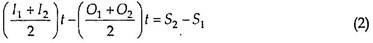
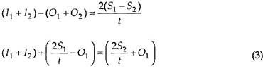
Let I1and I2 be the inflow rates and O1 and O2 be the outflow rates at the beginning and end of the time interval t. Let S1 be the storage in the beginning and S2 at the end of the time interval t.
These values can be substituted in the Eq. (1) as follows:

Now before further analysis could be carried out, following graphs are required:
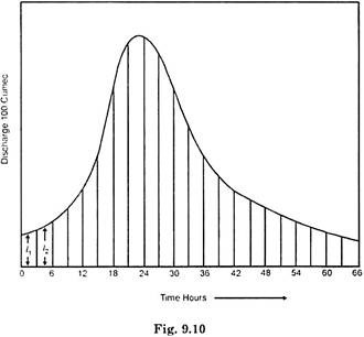
1. Inflow hydrograph.
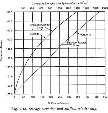
2. Elevation-outflow curve of the reservoir and
3. Elevation-storage curve of the reservoir.
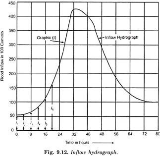
Inflow rate ordinates I1, I2, I3 etc. are read out from the inflow hydrograph at suitably chosen interval. Figure 9.10 shows an inflow hydrograph at 3 hours time interval and Fig. 9.12 shows an inflow hydrograph at 4 hours time interval.

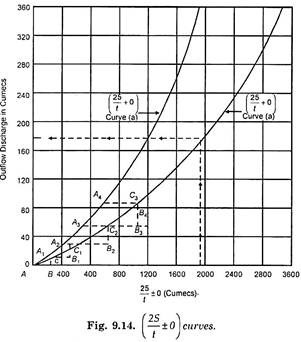
Now draw the curves between (2S/t ± O) versus outflow O. These curves are shown in Fig. 9.14. To draw these curves values of S and O for various values of reservoir elevation are read from elevation outflow and elevation storage curves shown in Fig. 9.13. Knowing S and O, values of (2S/t ± O) are found out and plotted against the corresponding outflow rates O as shown in Fig. 914. Here t is the any chosen time interval.
Now at the beginning both S1 and O1 are zero. By putting these values in Eq. (3), we get
I1 + I2 = 2S2 / t + O2
For first time interval t, the rates of inflow at the beginning and end are respectively I1, I2, I1 and I2 are read from the inflow hydrograph curve. Hence 2S2 / t + O2 is known.
From Fig. 9.14 (a) and (b) curves enter this value of 2S2 / t + O2 and get O2. For this value of O2 also find 2S2 / t – O2 from the same figure curve (a). Now apply Eq. (3) for the next time interval
(I2 + I3) = (2S2 / t – O2) = 2S3 /t + O3
In this equation again I2 and l3 are read from mass inflow curve and (2S2 / t – O2) as explained above. Hence (2S3 /t + O3) is known. From Fig. 9.12 find the value of O3 corresponding to the value of (2S3 /t + O3). Also find (2S3 /t – O3) corresponding to the value of O3. Similarly applying Eq. (3) for the next time interval, we get (I3 + I4) + (2S3 / t – O3) = (2S4 /t + O4).
From which (2S4 /t + O4) is known and the process is repeated for the complete period of flood.
Steps of Graphical Method:
1. Determine total inflow for the first time interval t from the inflow hydrograph. Enter this value as AB in Fig. 9.14.
2. Through B draw a vertical line to meet the curve 2S/t + O at point C. The point C represents the value of outflow at the end of the interval.
3. Through C draw a horizontal line A1CB1 cutting (2S/t – O) curve in point A1.
4. Now calculate the total inflow during second subsequent time interval t again from inflow hydrograph. Measure the total inflow from A1 on line A1CB1 and mark point B1.
5. Again draw a vertical ordinate from B1 to meet the curve (2S/t + O) a point C1 and repeat the procedure as stated in steps (3) and (4) until the entire flood is routed.
6. The outflow discharge at any time interval is given by the total vertical ordinate. The largest of these ordinates will indicate the value of the peak outflow rate. The spillways are designed based of the largest discharge.
7. After determining the outflow discharge at various intervals as described above, the reservoir water level for these can be determined from (Fig. 9.13) graph II.
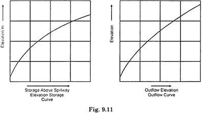
Elevation-Storage Curve and Elevation:
Outflow curve may be drawn separately as shown in Fig. 9.11. They can be drawn in one diagram also. Figure 9.13 shows elevation-storage curve and elevation-outflow curves on the same plot. Figure 9.13 shows cumulative storage on top n-axis time and outflow in bottom x-axis line.

One thing should be clearly understood that to account for the worst condition, the water surface in the reservoir is normally taken to be at the maximum conservation level or the full reservoir level and hence at the beginning of the first interval of time t, both storages and outflow O, are taken equal to zero.
Example:
Till following is the data of in inflow flood hydrograph whose flows in 100 cumecs have been recorded at 4 hours interval starting from zero hour on May 1, 2008 on a certain stream.

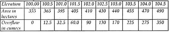
This flood is reaching a reservoir having un-gated spillways of which elevation area and Elevation outflow data are as follows:
It may be assumed that water level in the reservoir reaches the crest level (100.00) of the spillways at zero hours of May 1, 2008.
Determine the maximum reservoir level and maximum discharge over the spillway. Draw in flow and routed hydrograph indicating the reduction in peak flow and peak lag introduced due to routing.
Solution:
1. Draw the inflow hydrograph as shown in (Flood hydrograph) Fig. 9.12.
2. Draw elevation outflow curve as shown in Fig. 9.13 graph II.
3. Draw elevation storage curve as shown in Fig. 9.13 graph III. The starting level for the spillway is the crest level. For plotting this curve, volume between different contours is found by average area method.
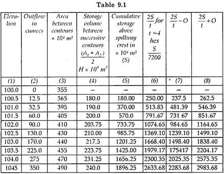
4. The values of 2S/t ± O have been found out in the Table 9.1.

5. The values of 2S/t – O (Col. 7) and 2S/t + O (Col. 8) each have been plotted against the outflow discharge (Col. 2) in Fig. 9.14.
The routing method is same as described under the graphical method. Instead of drawing vertical ordinates and doing purely graphically, the values can be tabulated as given in Table 9.2. The values of (2S/t – O) read each time and O are read each time from Fig. 9.14 curve (A). For different values 2S/t + O, the tabulated values are given here in the Table 9.2. Time interval is 4 hours.
The method of drawing vertical ordinates and corresponding horizontal ordinates are shown in Fig. 9.14.
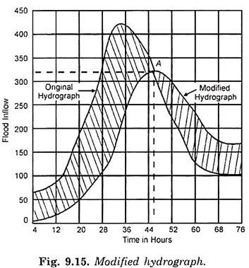
The inflow flood hydrograph and outflow flood hydrograph have been plotted together in Fig. 9.15.

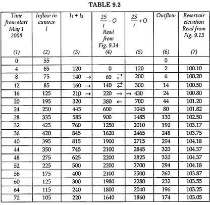
From Table 9.2 following results can be immediately noted.
i. Maximum reservoir level = 104.37 m.
ii. Maximum discharge over spillway = 320 cumecs.
iii. Reduction in peak discharge (Maximum inflow – Maximum outflow) (425 – 320) = 105 cumecs.
iv. Peak lag = Time for Maximum outflow – Time of Maximum inflow
= 46 – 32 = 14 hours.
2. Trial and Error Method of Routing Floods:
This is the most commonly used method of floods routing.
The method may be enumerated as per following steps:
i. Divide the inflow flood hydrograph into small intervals of time.
ii. Calculate the total inflow during the first time interval by multiplying the average inflow rates at the beginning and end of the period with time interval t.
i.e. (I1 + I2/ 2) t.
iii. The level of water at the start of the flood is known. It is taken at the crest level of the spillways.
iv. Assume a trial level of water in the reservoir at the end of the first period t.
v. Using elevation outflow-curve, calculate the outflow at the start and end of a particular time interval corresponding to water levels. When average value of outflow is multiplied by the time interval we get the net outflow during the period.
(O1 + O2 / 2) t
vi. Using the elevation storage curve find out the storage at the beginning and end of the time interval for the corresponding known water levels in the reservoir. Find out the difference in storages at the start and end of the time interval i.e. (S2 – S1). This difference represents the amount of flood stored in the reservoir during that period.
vii. Add the value of outflow obtained in step (v) to the value of storage obtained in (vi). The value should be equal to the total inflow during the period as calculated in step (ii). If the value i.e. sum of (v) and (vi) and (ii) are equal the assumed trial elevation of the reservoir is correct. If not assume some other value of water elevation and trial repeated, till value of sum of (v) and (vi) becomes very nearly equal to (ii).
viii. Repeat from steps ii to vii for all other little intervals till the flood is completely routed.
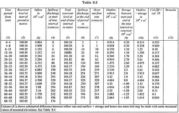
Solution by Trial and Error Method:
Make a table as shown in Table 9.3. Choose time interval of 4 hours and enter these values in column (1) of this table. In column (2) enter reservoir levels at start of each time interval. Calculate inflow of flood and enter its values in column 3 for each time interval.
Now using discharge-elevation curve of Fig. 9.13 find out the discharge over spillway at the start of each time interval corresponding to level of water in column (2) and enter them in column 4. Assume trial elevations, and enter them into column (5). For these trial elevations, calculate spillway discharge and enter them in column (6).
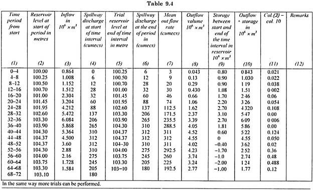
Determine the mean outflow rate by taking mean of column (4) and column (6). Enter mean values in column (7). Convert the values of column (7) into outflow volume in m3 and enter in column (8). The volume of outflow will be less than inflow volume so long as the peak of flood has not been routed. Once the peak of the flood has been routed, the volume of outflow exceeds the inflow volume. At this Lillie it is considered that maximum flood conditions have occurred.
Using storage elevation curve Fig. 9.13 find the storage capacity between the reservoir elevation at the beginning and end of the period. Enter all such values in column (9) Add columns (8) and (9) and enter in column (10). Figures in column (10) show the sum of outflow volume and storage capacity. Find out the difference between corresponding figures of column (3) and column (10) and enter in column (11). This difference between figures of column (3) and (20) should be negligible. Any remark may be written in column (12).
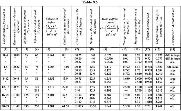
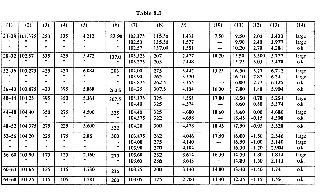
The trial and error method in Tables 9.3 and 9.4 can be replaced by Table 9.5 also. In Table 9.5 the reservoir elevation for each time interval is first adjusted before proceeding for subsequent time interval. Method of applying trials is better understood in Table 9.5 rather than Tables 9.3 and 9.4.
